Support Vector Machines: Mathematical derivation and use cases

There are various classification algorithms existing in the field of computational statistics and more robust, compute-time friendly algorithms are being invented as the study of machine learning progresses. However, for an algorithm invented in the 90’s, SVMs still hold a respectable place in real world applications and even academics. SVMs have performed surprisingly well when feature vectors are too large to cripple other algorithms. How do they handle very large feature vector spaces ? And why are they still popular?

With supervised learning algorithms, at some point the performance is pretty similar for all. What matters more is: how clean your data is, what features you have selected and what cost function you have picked. The nearest algorithm that can be compared to SVM is logistic regression and we will continue our mathematical derivation from logistic regression itself, slowly transgressing the Sigmoidal hypothesis function into a large margin classifier.

Alternative view of Logistic Regression:

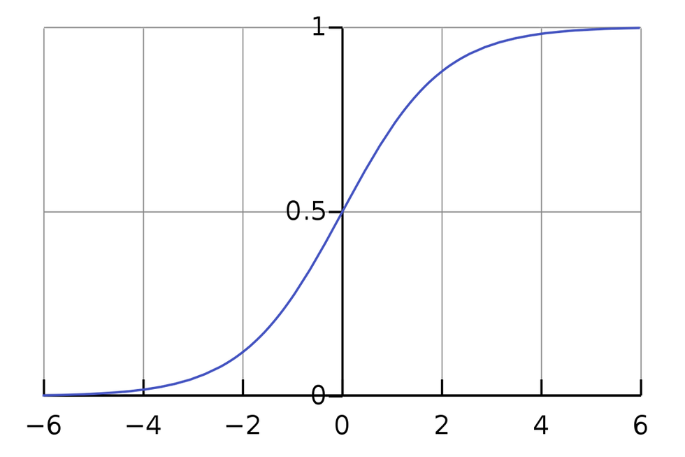
The hypothesis function of logistic regression is given by:

Where z = inner product of feature vector Θ and input vector x.

If result y = 1, we want h to be close to 1, or z to be greater than 0.

Similarly if y = 0, we want h to be close to 0, or z to be less than 0.

Fig 1: Sigmoidal Function

Cost function of Logistic regression:

where y is actual output and h is hypothesis function result.

When y = 1, the cost function becomes: J = -log(h)

Fig 2: J vs z graph when y = 1

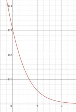
This function shows cost function J against z when y = 1. To build an SVM out of it, we have to redefine the cost function to follow this trend but in a simpler manner, so that J = 0 for z >= 1, and J is non zero for z < 1. This little modification makes the cost function computationally faster. The same trend is followed for y = 0, such as J = 0 for z <= -1 and J is non-zero otherwise.

Now that the cost function is modified, let’s take a look at the hypothesis function. Ideally it should be a step function but due to the modified cost function, the hypothesis function becomes as such:

h = 1 for z >= 1

h = 0 for z <= -1

A margin remains between 1 and -1 and this is why the SVM is called a Large Margin Classifier. This margin can be modified according to our wish and serves a purpose of actually ignoring the outliers present inside the margin.

The final cost function takes a form as follows:

The modified cost functions are Cost 1 and Cost 0 respectively and a constant C is added to amplify the cost function. The constant C is set to a moderate value and it helps the classifier to be more robust. If C is set too high, the decision boundary will try to include all points and leads to overfitting.

Use of Kernels:

Let’s see how SVM uses a Gaussian kernel to make the decision boundaries non-linear.

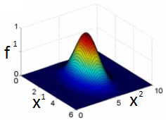
The input vector is modified with a Gaussian function to sort of change the input vector into something that the SVM can easily classify, so in that sense, the SVM itself does not form non linear decision boundaries but modifies the non-linear nature of the input into something that can be easily classified. Shown below is a Gaussian kernel in 2d space:

Fig 3: Gaussian Kernel

Till now we have seen some basic parameters and how they affect the functionality of SVMs. Now let’s get into the code.

SVM LINEAR KERNEL

import numpy as np
import matplotlib.pyplot as plt
from sklearn import svm, datasets

# import data
iris = datasets.load_iris()
X = iris.data[:, :2] # we only take the first two features.
y = iris.target

# we create an instance of SVM and fit out data.
C = 1.0 # SVM regularization parameter
svc = svm.SVC(kernel='linear', C=1,gamma=0).fit(X, y)

# create a mesh to plot in
x_min, x_max = X[:, 0].min() - 1, X[:, 0].max() + 1
y_min, y_max = X[:, 1].min() - 1, X[:, 1].max() + 1
h = (x_max / x_min)/100
xx, yy = np.meshgrid(np.arange(x_min, x_max, h), np.arange(y_min, y_max, h))

plt.subplot(1, 1, 1)
Z = svc.predict(np.c_[xx.ravel(), yy.ravel()])
Z = Z.reshape(xx.shape)
plt.contourf(xx, yy, Z, cmap=plt.cm.Paired, alpha=0.8)

plt.scatter(X[:, 0], X[:, 1], c=y, cmap=plt.cm.Paired)
plt.xlabel('Sepal length')
plt.ylabel('Sepal width')
plt.xlim(xx.min(), xx.max())
plt.title('SVC with linear kernel')
plt.show()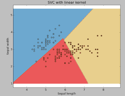

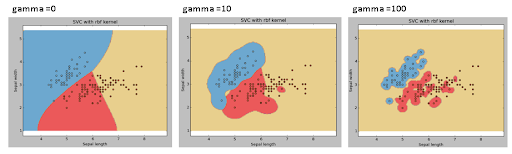
SVM RBF KERNEL

svc = svm.SVC(kernel='rbf', C=1,gamma=0).fit(X, y)

Gamma: Kernel coefficient for ‘rbf’, ‘poly’ and ‘sigmoid’. Higher the value of gamma, will try to exactly fit the as per training data set i.e. generalization error and cause overfitting problem.

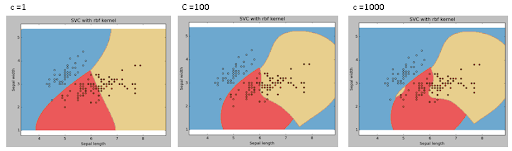
C: Penalty parameter C of the error term. It also controls the trade-off between smooth decision boundaries and classifying the training points correctly.

Let’s go through what we have learnt in this process:

• SVM helps us fit very high dimensional data, proving its advantage over Logistic Regression.

• Adding non-linear kernels helps us to fit non-linear data.

• Increasing the value of constant C leads to the model becoming more complex, helping it to fit more complex data points. However if C is too large, the model will train itself to include outliers too, leading to overfitting. So a moderate value of C is to be chosen.

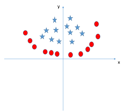
Practice Problem…

Determine the kernel function for this image and let me know in the comments section.

Edited by coolman-spaceman