Role of the Activation Function in a Neural Network Model
- Priyanka P. Pattnaik
- Apr 30, 2020
- 4 min read
In a neural network, numeric data points, called inputs, are fed into the neurons in the input layer. Each neuron has a weight, and multiplying the input number with the weight gives the output of the neuron, which is transferred to the next layer.
The activation function is a mathematical “gate” in between the input feeding the current neuron and its output going to the next layer. It can be as simple as a step function that turns the neuron output on and off, depending on a rule or threshold. Or it can be a transformation that maps the input signals into output signals that are needed for the neural network to function.
Increasingly, neural networks use non-linear activation functions, which can help the network learn complex data, compute and learn almost any function representing a question, and provide accurate predictions.

3 Types of linear Activation Functions
1. Binary Step Function
A binary step function is a threshold-based activation function. If the input value is above or below a certain threshold, the neuron is activated and sends exactly the same signal to the next layer.

The problem with a step function is that it does not allow multi-value outputs—for example, it cannot support classifying the inputs into one of several categories.
2. Linear Activation Function
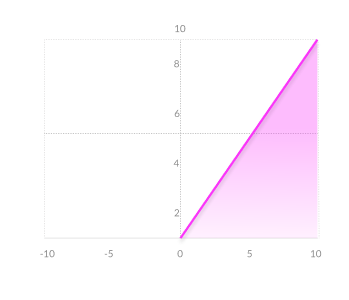
A linear activation function takes the form: A = cx

It takes the inputs, multiplied by the weights for each neuron, and creates an output signal proportional to the input. In one sense, a linear function is better than a step function because it allows multiple outputs, not just yes and no.
However, a linear activation function has two major problems:
1. Not possible to use backpropagation (gradient descent) to train the model—the derivative of the function is a constant, and has no relation to the input, X. So it’s not possible to go back and understand which weights in the input neurons can provide a better prediction.
2. All layers of the neural network collapse into one—with linear activation functions, no matter how many layers in the neural network, the last layer will be a linear function of the first layer (because a linear combination of linear functions is still a linear function). So a linear activation function turns the neural network into just one layer.
A neural network with a linear activation function is simply a linear regression model. It has limited power and the ability to handle complexity varying parameters of input data.
3. Non-Linear Activation Functions
Modern neural network models use non-linear activation functions. They allow the model to create complex mappings between the network’s inputs and outputs, which are essential for learning and modeling complex data, such as images, video, audio, and data sets which are non-linear or have high dimensionality.
Almost any process imaginable can be represented as a functional computation in a neural network, provided that the activation function is non-linear.
Non-linear functions address the problems of a linear activation function:
They allow backpropagation because they have a derivative function which is related to the inputs.
They allow “stacking” of multiple layers of neurons to create a deep neural network. Multiple hidden layers of neurons are needed to learn complex data sets with high levels of accuracy.
7 Common Nonlinear Activation Functions and How to Choose an Activation Function
3.1 Sigmoid / Logistic
Advantages
Smooth gradient, preventing “jumps” in output values.
Output values bound between 0 and 1, normalizing the output of each neuron.
Clear predictions—For X above 2 or below -2, it tends to bring the Y value (the prediction) to the edge of the curve, very close to 1 or 0. This enables clear predictions.
Disadvantages
Vanishing gradient—for very high or very low values of X, there is almost no change to the prediction, causing a vanishing gradient problem. This can result in the network refusing to learn further, or being too slow to reach an accurate prediction.
Outputs not zero centered.
Computationally expensive

3.2 TanH / Hyperbolic Tangent
Advantages
Zero centered—making it easier to model inputs that have strongly negative, neutral, and strongly positive values.
Otherwise like the Sigmoid function.
Disadvantages
Like the Sigmoid function

3.3 ReLU (Rectified Linear Unit)
Advantages
Computationally efficient—allows the network to converge very quickly
Non-linear—although it looks like a linear function, ReLU has a derivative function and allows for backpropagation
Disadvantages
The Dying ReLU problem—when inputs approach zero or are negative, the gradient of the function becomes zero, the network cannot perform backpropagation and cannot learn.

3.4 Leaky ReLU
Advantages
Prevents dying ReLU problem—this variation of ReLU has a small positive slope in the negative area, so it does enable backpropagation, even for negative input values
Otherwise like ReLU
Disadvantages
Results not consistent—leaky ReLU does not provide consistent predictions for negative input values.

3.5 Parametric ReLU
Advantages
Allows the negative slope to be learned—unlike leaky ReLU, this function provides the slope of the negative part of the function as an argument. It is, therefore, possible to perform backpropagation and learn the most appropriate value of α.
Otherwise like ReLU
Disadvantages
May perform differently for different problems.

3.6 Softmax
Advantages
Able to handle multiple classes only one class in other activation functions—normalizes the outputs for each class between 0 and 1, and divides by their sum, giving the probability of the input value being in a specific class.
Useful for output neurons—typically Softmax is used only for the output layer, for neural networks that need to classify inputs into multiple categories.

3.7 Swish
Swish is a new, self-gated activation function discovered by researchers at Google. According to their paper, it performs better than ReLU with a similar level of computational efficiency. In experiments on ImageNet with identical models running ReLU and Swish, the new function achieved top -1 classification accuracy 0.6-0.9% higher.


.png)


Comments